Capacity planning: ESA vs OSA, what really changes

An OSA sizing sheet cannot become an ESA sheet by renaming two columns. OSA reasons in disk groups, cache, and capacity. ESA reasons in storage pools, claimed raw capacity, System Usage, and RAID Factor. VCF 9.1 adds an Effective Capacity view that makes this new arithmetic explicit—provided Auto-RAID is in use.

Nordwind Logistics must arbitrate one budget across three clusters: cl-fret-prod-01, ESA with 8 hosts; cl-fret-dens-01, ESA with 4 hosts and a memory-tiering candidate; and cl-fret-legacy-01, OSA with 6 hosts and 2 disk groups per host. The last is a comparison point, not a target architecture.

TL;DR

• In ESA 9.1, the baseline is Total Usable Capacity = (Total Raw Capacity - System Usage) / RAID Factor.
• The old operations reserve and host rebuild reserve lines are gone from the 9.1 interface; do not reinsert them as the current method.
• Compression, deduplication, thin provisioning, and snapshots are measured separately, not one promised reduction ratio.
• An NVMe device reserved for memory tiering can no longer contribute to the storage pool: sizing must count slots, not only terabytes.

First, stop translating line by line

In OSA, each disk group contains one flash cache device and one or more capacity devices. In ESA, devices claimed by vSAN form one storage pool per host and all contribute to capacity and performance.

That difference makes several habits obsolete: retaining a cache line, carrying forward a legacy reserve, or applying an assumed reduction rate. An ESA sheet must restart from the objects exposed by the current version.

OSA line	ESA 9.1 line	Treatment
cache per disk group	no direct equivalent	remove the line; inventory the storage pool
capacity devices	every NVMe device claimed by vSAN	add claimed raw capacity
operations / host rebuild reserve	absent from the 9.1 interface	do not use as the current formula
percentage slack rule	no loaded rule	set and qualify a local margin
global data reduction	separate Space Efficiency measures	observe, do not predict
usable capacity	Effective Capacity	apply the published formula

RECONSTITUTION: this table assembles several official pages. No reviewed TechDocs 9.1 page directly compares OSA and ESA sizing methods.

The Effective Capacity formula

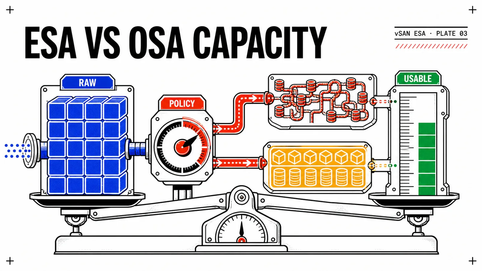
VCF 9.1 documentation publishes this equation:

Total Usable Capacity = (Total Raw Capacity - System Usage) / RAID Factor

• Total Raw Capacity adds the volumes of claimed drives.
• System Usage includes global metadata, filesystem overhead, ESA object overhead, deduplication overhead, and system reservations.
• RAID Factor comes from the cluster’s actual configuration.

Broadcom’s example calculates (40 - 14.5) / 1.5 and returns 17 TB usable. The 14.5 TB of System Usage belongs only to that example: the reviewed documentation gives no method for extrapolating it by cluster size or host count.

RÉSULTAT_ATTENDU: the sizing sheet and Effective Capacity view converge when they use the same raw capacity, System Usage, and RAID Factor. If the target view has not yet been collected, the cell must say “collect from the platform” instead of carrying an estimate.

Auto-RAID supplies the factor, not the requirement

VCF 9.1’s Effective Capacity view requires Auto-RAID. For a standard cluster, Broadcom publishes:

Size	Applied policy	RAID Factor
fewer than 3 hosts	FTT=0	1.0x
3 to 5 hosts	FTT=1, RAID-5	1.5x
6 hosts or more	FTT=2, RAID-6	1.5x

For a stretched cluster, inter-site mirroring raises the factor to 3.0x from 3 hosts per site with local RAID-5 or RAID-6. A 2-node cluster uses mirroring with local FTT=0 and a 2.0x factor.

New clusters use Auto-RAID by default. Existing clusters retain their policy and receive a health alert recommending migration. Host count is therefore never sufficient evidence of effective state.

The ESA RAID-5/6 write path explains why these policies become credible defaults. Capacity planning must remain agnostic: it reads the factor actually applied.

What replaces legacy reserves

In vSAN 8.0, operations reserve held space for internal operations and host rebuild reserve for repair after losing one host. The former included an additional 5% buffer. That model explains older sheets, but Broadcom says these mechanisms are no longer in the 9.1 interface because they belonged to the previous capacity-management approach.

This does not mean operations can consume every advertised byte without discipline. It means local operating margin no longer comes from copying an 8.0 reserve into the 9.1 formula.

HYPOTHÈSE_DE_DESIGN: Nordwind keeps an operating margin separate from the vendor formula and documents it as an internal decision. It is never presented as a Broadcom prerequisite.

Measure space efficiency without buying it in advance

VCF 9.1 changes ESA compression from LZ4 to ZSTD. Broadcom describes ZSTD as potentially providing better compression with modest CPU cost, without publishing a figure. Global deduplication becomes cluster-wide and post-process; it is unsupported on stretched and 2-node clusters.

The Space Efficiency view separates data-reduction ratio, thin-provisioning savings, and snapshot savings. Preserve that separation in the worksheet. Combining compression and deduplication into one ratio before observation hides risk.

The conservative method is straightforward:

1. buy against usable capacity without an unobserved gain;
2. collect each ratio after the workload stabilises;
3. use the trend for the next forecast;
4. verify any data-specific gain or CPU-cost assertion on a test platform.

NVMe slots close the equation

A device already claimed by vSAN cannot serve memory tiering. The NVMe memory tier requires a local, compatible, unclaimed device; 9.1 mirroring needs a second device of compatible size.

The cl-fret-dens-01 trade-off must follow this order:

• define minimum usable capacity and resilience;
• count NVMe devices required by the storage pool;
• then reserve the memory-tier slot or slots;
• recalculate ESA raw capacity after that reservation;
• compare final cost with adding DRAM or chassis.

The physical constraint prevents a fictional business case where the same NVMe device doubles memory while remaining available to storage.

This approach completes VCF 9.1 infrastructure efficiency and TCO: density is valuable only when sacrificed resources remain visible in the same economic model.

Conclusion

ESA does not make capacity planning vaguer; it recentres it on observable values. The formula is publishable without a lab. Local System Usage, margin, and ratios simply remain identified as data to verify on the target platform.

Primary sources: VCF 9.1 Effective Capacity, new capacity view, VCF 9.1 Auto-RAID, and VCF 9.1 compression and deduplication.